Quasi-Newton method
In optimization, quasi-Newton methods (also known as variable metric methods) are algorithms for finding local maxima and minima of functions. Quasi-Newton methods are based on Newton's method to find the stationary point of a function, where the gradient is 0. Newton's method assumes that the function can be locally approximated as a quadratic in the region around the optimum, and use the first and second derivatives to find the stationary point.
In Quasi-Newton methods the Hessian matrix of second derivatives of the function to be minimized does not need to be computed. The Hessian is updated by analyzing successive gradient vectors instead. Quasi-Newton methods are a generalization of the secant method to find the root of the first derivative for multidimensional problems. In multi-dimensions the secant equation is under-determined, and quasi-Newton methods differ in how they constrain the solution, typically by adding a simple low-rank update to the current estimate of the Hessian.
The first quasi-Newton algorithm was proposed by W.C. Davidon, a physicist working at Argonne National Laboratory. He developed the first quasi-Newton algorithm in 1959: the DFP updating formula, which was later popularized by Fletcher and Powell in 1963, but is rarely used today. The most common quasi-Newton algorithms are currently the SR1 formula (for symmetric rank one), the BHHH method, the widespread BFGS method (suggested independently by Broyden, Fletcher, Goldfarb, and Shanno, in 1970), and its low-memory extension, L-BFGS. The Broyden's class is a linear combination of the DFP and BFGS methods.
The SR1 formula does not guarantee the update matrix to maintain positive-definiteness and can be used for indefinite problems. The Broyden's method does not require the update matrix to be symmetric and it is used to find the root of a general system of equations (rather than the gradient) by updating the Jacobian (rather than the Hessian).
Contents |
Description of the method
As in Newton's method, one uses a second order approximation to find the minimum of a function  . The Taylor series of around an iterate is:
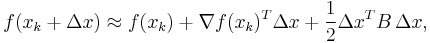
where ( ) is the gradient and
  an approximation to the Hessian matrix. The gradient of this approximation (with respect to
  ) is
) is

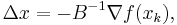
and setting this gradient to zero provides the Newton step:
The Hessian approximation is chosen to satisfy

which is called the secant equation(the Taylor series of the gradient itself). In more than one dimension is under determined. In one dimension, solving for and applying the Newton's step with the updated value is equivalent to the secant method. Various methods are used to find the solution to the secant equation that is symmetric ( ) and closest to the current approximate value
  according to some metric
 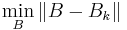 . An approximate initial value of
  is often sufficient to achieve rapid convergence. The unknown
  is updated applying the Newton's step calculated using the current approximate Hessian matrix
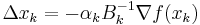 , with
  chosen to satisfy the Wolfe conditions;
 ;
;- The gradient computed at the new point
 , and
, and
is used to update the approximate Hessian  , or directly its inverse
  using the Sherman-Morrison formula.
- A key property of the BFGS and DFP updates is that if is positive definite and
 is chosen to satisfy the Wolfe conditions then is also positive definite.
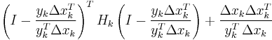
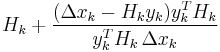
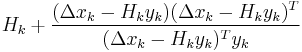
The most popular update formulas are:
| Method |  |
 |
|---|---|---|
| DFP |  |
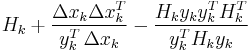 |
| BFGS | 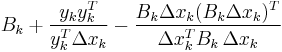 |
 |
| Broyden | 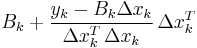 |
 |
| Broyden family | ![(1-\varphi_k) B_{k%2B1}^{BFGS}%2B \varphi_k B_{k%2B1}^{DFP}, \qquad \varphi\in[0,1]](/2012-wikipedia_en_all_nopic_01_2012/I/fa0b40f635e471dac81b5ee2f76acda1.png) |
|
| SR1 | 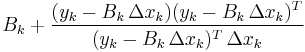 |
 |
Example algorithm using matlab
%***********************************************************************%
% Usage: [x,Iter,FunEval,EF] = Quasi_Newton (fun,x0,MaxIter,epsg,epsx)
%         fun: name of the multidimensional scalar objective function
%              (string). This function takes a vector argument of length
%              n and returns a scalar.
%          x0: starting point (row vector of length n).
%     MaxIter: maximum number of iterations to find a solution.
%        epsg: maximum acceptable Euclidean norm of the gradient of the
%              objective function at the solution found.
%        epsx: minimum relative change in the optimization variables x.
%           x: solution found (row vector of length n).
%        Iter: number of iterations needed to find the solution.
%     FunEval: number of function evaluations needed.
%          EF: exit flag,
%              EF=1: successful optimization (gradient is small enough).
%              EF=2: algorithm converged (relative change in x is small
%                    enough).
%              EF=-1: maximum number of iterations exceeded.

%  C) Quasi-Newton optimization algorithm using (BFGS)                  %

function [x,i,FunEval,EF]= Quasi_Newton (fun, x0, MaxIter, epsg, epsx)
%   Variable Declaration
 xi        = zeros(MaxIter+1,size(x0,2));
 xi(1,:)   = x0;
 Bi        = eye(size(x0,2));

%  CG algorithm
FunEval = 0;
EF = 0;

  for i = 1:MaxIter

      %Calculate Gradient around current point
      [GradOfU,Eval] =  Grad (fun, xi(i,:));
      FunEval        =  FunEval + Eval;       %Update function evaluation

      %Calculate search direction
      di             = -Bi\GradOfU ;

      %Calculate Alfa via exact line search
      [alfa, Eval]   =  LineSearchAlfa(fun,xi(i,:),di);
      FunEval        =  FunEval + Eval;       %Update function evaluation

      %Calculate Next solution of X
      xi(i+1,:)      =  xi(i,:) + (alfa*di)';

      % Calculate Gradient of X on i+1
      [Grad_Next, Eval] =  Grad (fun, xi(i+1,:));
      FunEval           =  FunEval + Eval;       %Update function evaluation

      %Calculate new Beta value using BFGS algorithm
      Bi                =  BFGS(fun,GradOfU,Grad_Next,xi(i+1,:),xi(i,:), Bi);

      % Calculate maximum acceptable Euclidean norm of the gradient
      if norm(Grad_Next,2) < epsg
          EF        = 1;
          break
      end

      % Calculate minimum relative change in the optimization variables
      E            =   xi(i+1,:)- xi(i,:);
      if norm(E,2) < epsx
          EF       = 2;
          break
      end
  end
  % report optimum solution
   x    = xi(i+1,:);

  if i == MaxIter
  % report Exit flag that MaxNum of iterations reach
     EF =  -1;
  end

  % report MaxNum of iterations reach
  Iter  = i;

end

%***********************************************************************%
% Broyden, Fletcher, Goldfarb and Shanno (BFGS) formula
%***********************************************************************%
function  B  = BFGS(fun,GradOfU,Grad_Next,Xi_next,Xi,Bi)

 % Calculate Si term
  si               =  Xi_next   - Xi;

 % Calculate Yi term
  yi               =  Grad_Next - GradOfU;
 %
 % BFGS formula (Broyden, Fletcher, Goldfarb and Shanno)
 %
  B   =  Bi - ((Bi*si'*si*Bi)/(si*Bi*si')) + ((yi*yi')/(yi'*si'));

end
See also
References
- Bonnans, J. F., Gilbert, J.Ch., Lemaréchal, C. and Sagastizábal, C.A. (2006), Numerical optimization, theoretical and numerical aspects. Second edition. Springer. ISBN 978-3-540-35445-1.
- William C. Davidon, Variable Metric Method for Minimization, SIOPT Volume 1 Issue 1, Pages 1–17, 1991.
- Fletcher, Roger (1987), Practical methods of optimization (2nd ed.), New York: John Wiley & Sons, ISBN 978-0-471-91547-8.
- Nocedal, Jorge & Wright, Stephen J. (1999). Numerical Optimization. Springer-Verlag. ISBN 0-387-98793-2.
- Press, WH; Teukolsky, SA; Vetterling, WT; Flannery, BP (2007). "Section 10.9. Quasi-Newton or Variable Metric Methods in Multidimensions". Numerical Recipes: The Art of Scientific Computing (3rd ed.). New York: Cambridge University Press. ISBN 978-0-521-88068-8. http://apps.nrbook.com/empanel/index.html#pg=521.
|
|||||||||||||||||||||||||||||||||||||||||||||||||||||||||||||||||||||||||||||||||||||||||